Recently I came across the requirement to monitor traffic for a few devices behind Ubiquiti EdgeRouters, so I put together the following method which is described here for future reference. I am using iptables to collect byte counts and poll this data through SSH from a monitoring server. The collected data gets saved in a round robin database and output as a graph using Tobias Oetiker’s geat RRDtool.

Counting bytes

Create a new Firewall Policy (aka. iptables chain) on the EdgeRouter and add one rule per device and direction (in/out) to be monitored. The rule should pass along all traffic, all we are interested in, is the byte count. To select the correct device, I chose MAC addresses for outgoing and statically assigned DHCP addresses for incoming.

# show firewall name TRAFFIC_ACCT
default-action accept
description "Traffic accounting"
rule 1 {
  action accept
  description S01
  log disable
  protocol all
  source {
    mac-address 00:90:xx:xx:xx:xx
  }
}
rule 2 {
  action accept
  description S02
  log disable
  protocol all
  source {
    mac-address 00:90:xx:xx:xx:xx
  }
}
rule 5 {
    action accept
    description S01_in
    destination {
        address 10.200.0.58
    }
    log disable
    protocol all
}
rule 6 {
    action accept
    description S02_in
    destination {
        address 10.200.0.27
    }
    log disable
    protocol all
}

Storing the data

On your monitoring server create a database using RRDtool.

rrdtool create /var/rrd/devices.rrd \
  DS:S01:COUNTER:600:U:U \
  DS:S02:COUNTER:600:U:U \
  DS:S01_in:COUNTER:600:U:U  \
  DS:S02_in:COUNTER:600:U:U  \
  RRA:AVERAGE:0.5:1:576 \
  RRA:AVERAGE:0.5:6:720 \
  RRA:AVERAGE:0.5:24:720 \
  RRA:AVERAGE:0.5:288:730

This creates a round robin database with 4 datasources, using the “COUNTER” data source type for each of them. I defined a 600 second (10 minutes) heartbeat value, meaning data that is collected in this timeframe is still considered valid for this data point. Since I am collecting new values every 5 minutes, this gives a big enough margin for occasional slower connection times to the remote devices form the monitoring server.

Collecting data

To collect data, create a cronjob on your monitoring system connecting to the EdgeRouter via SSH and reading out the byte counts via iptables.

# cat /etc/cron.d/traffic_acct
*/5 * * * * root /usr/bin/rrdupdate /var/rrd/devices.rrd N:$(ssh -q user@edge.router sudo iptables -L TRAFFIC_ACCT -v -n -x | head -n -1 | tail -n +3 | awk '{print $2}' | xargs echo | sed 's/ /:/g') && /usr/local/bin/rrd_graph.sh >> /dev/null 2>&1

This command is made up of several parts. First it defines that cron should run it every 5 minutes as user “root”. The rrdupdate part instructs rrdtool to feed new data into the RRD file we created previously. Data updates are to be provided as integers separated by “:” and preceded by a timestamp. In this particular case I am using “N” as the time-value, this defaults to the current timestamp. The next part is a bash inline command substitution. It connects to the remote device via SSH and runs iptables and then formatting the output in a way rrdupdate can read. -L TRAFFIC_ACCT selects the correct chain we are interested in, -v -n -x uses verbose mode, numeric output (don’t resolve DNS names) and exact value of byte counters instead of only the rounded number in K’s (multiples of 1000) M’s (multiples of 1000K) or G’s (multiples of 1000M). The last part cuts off the first and last lines, which I’m not interested in and reformats every line to one single line of output substituting spaces with “:”.

After the data collection and updating is done, the cronjob runs a second script (rrd_graph.sh) which creates/updates the graph which can then be displayed on a webpage.

Creating the graph

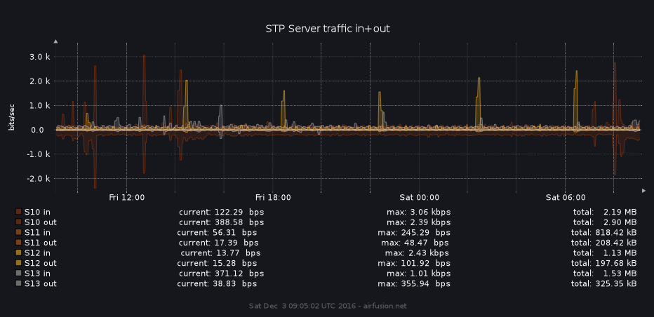
As one can see in the previous command, the graph itself is created using a shell script which is run each time after the round robin database is updated. Here is an example for a nice looking graph using the collected data. I’ve opted for SVG (scalable vector graphics) so it is possible to manually zoom into the graph without loosing quality (e.g. on a cellphone) when displayed on a webpage.

#!/bin/sh

DB=/var/rrd/devices.rrd
RRDTOOL=/usr/bin/rrdtool
OUT=/var/www/traffic/images/devices.svg

$RRDTOOL graph $OUT --start -1d \
    -E -w 800 -h 200 --border=0 --disable-rrdtool-tag \
    -a SVG --title="Traffic in+out" \
    -c MGRID#E0E1E550 --no-minor -c ARROW#B0B0B0 \
    -c CANVAS#16161D -c FONT#FFFFFF -c BACK#16161D \
    --vertical-label "bits/sec" \
    --watermark "$(date) - airfusion.net" \
    --font TITLE:10:'/usr/share/fonts/truetype/droid/DroidSansMono.ttf' \
    --font AXIS:8:'/usr/share/fonts/truetype/droid/DroidSansMono.ttf' \
    --font LEGEND:8:'/usr/share/fonts/truetype/droid/DroidSansMono.ttf' \
    --font UNIT:7:'/usr/share/fonts/truetype/droid/DroidSansMono.ttf' \
    --font WATERMARK:7:'/usr/share/fonts/truetype/droid/DroidSansMono.ttf' \
    DEF:S01=$DB:S01:AVERAGE \
    DEF:S02=$DB:S02:AVERAGE \
    DEF:S01_in=$DB:S01_in:AVERAGE \
    DEF:S02_in=$DB:S02_in:AVERAGE \
    CDEF:S01b=S01,8,*,-1,* \
    CDEF:S02b=S02,8,*,-1,* \
    CDEF:S01b_d=S01,8,* \
    CDEF:S02b_d=S02,8,* \
    CDEF:S01b_in=S01_in,8,* \
    CDEF:S02b_in=S02_in,8,* \
    VDEF:S01total=S01,TOTAL \
    VDEF:S02total=S02,TOTAL \
    VDEF:S01total_in=S01_in,TOTAL \
    VDEF:S02total_in=S02_in,TOTAL \
    LINE1:S01b_in#92380690:"S01 in  "\
    AREA:S01b_in#92380630: \
    GPRINT:S01b_in:LAST:"current\: %4.2lf %sbps" \
    GPRINT:S01b_in:MAX:"max\: %4.2lf %sbps" \
    GPRINT:S01total_in:"total\:%7.2lf %sB \j" \
    LINE1:S01b#92380690:"S01 out"\
    AREA:S01b#92380630: \
    GPRINT:S01b_d:LAST:"current\: %4.2lf %sbps" \
    GPRINT:S01b_d:MAX:"max\: %4.2lf %sbps" \
    GPRINT:S01total:"total\:%7.2lf %sB \j" \
    LINE1:S02b_in#ce610790:"S02 in  "\
    AREA:S02b_in#ce610730: \
    GPRINT:S02b_in:LAST:"current\: %4.2lf %sbps" \
    GPRINT:S02b_in:MAX:"max\: %4.2lf %sbps" \
    GPRINT:S02total_in:"total\:%7.2lf %sB \j" \
    LINE1:S02b#ce610790:"S02 out"\
    AREA:S02b#ce610730: \
    GPRINT:S02b_d:LAST:"current\: %4.2lf %sbps" \
    GPRINT:S02b_d:MAX:"max\: %4.2lf %sbps" \
    GPRINT:S02total:"total\:%7.2lf %sB \j" \
    HRULE:0#E0E1E595 \

Graph Script breakdown

First we define a few variables for local paths to the RRD file, the rrdtool binary and our output file. The next part starts the actual definition of the graph.

--start -1d defines the timeframe that should be shown. This is also used for each of the calculated values below the image. In this case I’ve opted for 24 hours of data.

-E -w 800 -h 200 --border=0 --disable-rrdtool-tag this sets some options for the resulting image, in particular it uses slope mode (-E, you can read more about this option in the rrdgraph man page), sets width and height (which might not mean much, since we’re creating vector data anyway), disables the border and the rrdtool watermark to get a cleaner look for the resulting graph.

-a SVG --title="Traffic in+out" defines the output format and sets a title for the image.

-c MGRID#E0E1E550 --no-minor -c ARROW#B0B0B0 sets gridline colors, disables some of the in-beween lines and the color for the arrows on the upper and right hand side of the y- and x-axis respectively. Color definitions are in HEX format with an optional added 4th character pair at the end defining the transparency.

-c CANVAS#16161D -c FONT#FFFFFF -c BACK#16161D this line defines the color for the background and the text in the resulting image.

--vertical-label "bits/sec" this is the label that gets applied to the y-axis.

--watermark "$(date) - airfusion.net" the watermark will be displayed on the bottom of the image and can be any text you want. I added the current timestamp, so it would always be apparent at which time the graph was actually created, when looking at the image.

The next 5 lines define the font size and family for various parts of the graph image.

DEF is the input, it selects all available datapoints (in and out for each device) from our rrd file and assigns it to local “variables” (S01, S01_in etc.) using the “AVERAGE” consolidation function.

CDEF:S01b=S01,8,*,-1,* computes the data in S01 using reverse polish notation and assigns it to S01b (“b” for bits). First it takes the value and mulitiplies it by 8 , thus converting bytes to bits and then multiplies by -1 to reverse the number, so in the resulting graph all traffic going out (aka. upload) is shown on the negative y-axis. This helps visually separating incoming and outgoing traffic in a more meaningful way. The next line does the same for S02 data.

CDEF:S01b_d=S01,8,* this part takes S01 data and only converts it to bits, without converting it to negative. The value in the resulting S01b_d (“d” for display) variable is then used in the legend below the graph. We don’t want negative numbers there for our display. Again, the next line does the equivalent for S02.

CDEF:S01b_in=S01_in,8,* converts S01_in data to bytes for graphing purposes, this should be fairly obvious by now. As does the next line for S02_in.

VDEF:S01total=S01,TOTAL takes S01 data and sums it up for the selected timeframe. The same goes for the next 3 lines for S02, S01_in and S02_in. These values will then be displayed below the image.

LINE1:S01b_in#92380690:"S01 in " creates the first actual line on the graph using a brownish color from the values of our calculated S01b_in variable. The last part is the label that gets added to the legend under the graph, including some spaces at the end in an attempt to line up the text a bit better.

AREA:S01b_in#92380630: takes the same data as previously but drawing it as a transparent area under the line created previously. This just gives a nice visual effect and serves no other purpose.

GPRINT:S01b_in:LAST:"current\: %4.2lf %sbps" this line creates the “current” value for our legend under the graph. It uses the “LAST” datapoint from the S01b_in variable and prints it out using a number width of 4 and 2 decimal places as a long float. %s means rrdtool will take the value and replace it by the appropriate SI magnitude unit and the value will be scaled accordingly (123456 -> 123.456 k). Lastly we add the suffix “bps”. The next 2 lines do the same for the maximum and total values.
The next few blocks are just the equivalent for S01b (S01 outgoing), S02b_in (S02 incoming) and S02b (S02 outgoing).

HRULE:0#E0E1E595 just draws a slightly more visible line through 0 on the y-axis to better separate incoming from outgoing traffic.